In my thesis I studied stratified randomization and it’s consequences for modelling. In this post I will try to distill some of my work. This first blog post describes stratified randomization and its conseqeunces for modelling.

Randomization

In a clinical trial, we want to single out the causal effect of treatment on the outcome. One way of ensuring that we can estimate a causal effect is by randomizing treatment to the study participants to balance the baseline covariates across treatment groups on average. That is, we aim for the two treatment groups to be comparable in all matters except treatment.

There are many ways of randomizing treatment, but the simplest is to flip a fair coin to allocate treatment each time a participant enrolls in a study. This works well for large studies, but for small studies, there can be a significant risk of an imbalanced treatment allocation.

To avoid this, we may enforce balance by using blocked randomization. Blocked randomization works by choosing an even number $k$ and then allocating treatment by drawing a random permutation of $k/2$ treated and $k/2$ controls for every $k$ participants enrolling in your study. The block size $k$ is typically chosen to be 4, 6, 8, or randomized among these.

But even when treatment is forced to be balanced at all times, covariate imbalance across treatment is only guaranteed in expectation, and this may yield serious consequences for inference. In the extreme case, we may allocate all males to control and all females to treatment, but even in the non-extreme case, a large imbalance across treatment for a variable that is prognostic of the outcome can mar the purpose of randomization and lead to unnecessary uncertainty.

Nearly all clinical trials conducted across various locations stratify by site to facilitate easier administration and data management. Additionally, many of these trials also stratify based on other baseline variables.

Stratified Randomization

Stratified randomization solves the issue of covariate imbalance by stratifying the randomization onto levels of certain prognostic baseline covariates. These levels are called strata. As an example, you might use blocked randomization within males and females separately to balance the distribution of sex across treatment, and typically, you only stratify on a few variables.

To observe the consequences of stratified randomization for modeling, we posit the following trial in which we expect sex to be prognostic of the outcome and randomize patients within sex using blocked randomization. Let $Y$ denote the continuous outcome, $X$ denote sex, and $A$ denote a binary treatment variable where we target a 1:1 allocation.

Inspired by (Kahan and Morris 2012) we posit the following DGP’s. For each $i = 1, \dots, 100$, let

\[\begin{align*} &X_i \sim \text{Bernoulli}(1/2)\\ &A_i \sim \text{Bernoulli}(1/2)\\ &Y_i \mid X_i, A_i \sim \alpha + \beta_A A_i + \beta_X X_i \end{align*}\]

and

\[\begin{align*} &X_i \sim \text{Bernoulli}(1/2)\\ &A_i \sim \text{Stratified block randomization on } X \text{ with a block size of 4} \\ &Y_i \mid X_i, A_i \sim \alpha + \beta_A A_i + \beta_X X_i \end{align*}\]

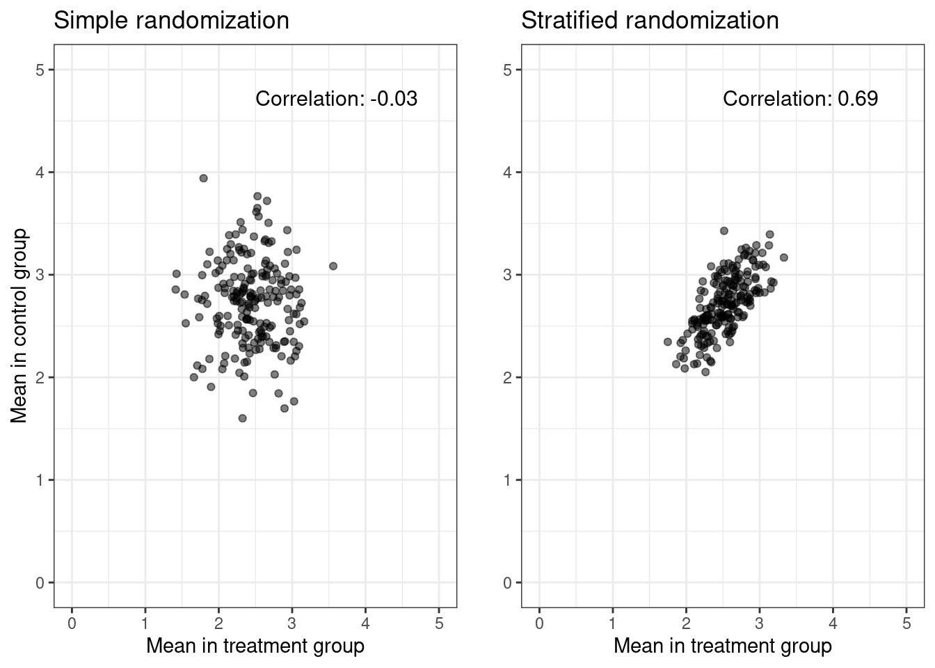
In the figure below, we simulate $N = 200$ datasets, each of size $n = 100$ with parameters $(\alpha = 0, \beta_A = 0.2, \beta_X = 0.5)$, and plot the treatment specific means against each other.

Code

# Kahan, B. C., & Morris, T. P. (2011). Improper analysis of trials randomised
# using stratified blocks or minimisation. Statistics in Medicine, 31(4),
# 328–340. doi:10.1002/sim.4431 
library(tidyverse)
library(blockrand)
library(patchwork)
library(gridExtra)

# Number of datasets
N = 200

# Size of each dataset
n_size = 100

sim_data = function(n_size, rand_type = 0, pX = 0.5) {

    # Simulate binary baseline covariate / the balancing variable
    sex = rbinom(n_size, 1, pX)

    # Simple randomization
    A_simple = rbinom(n_size, 1, 0.5)

    # Stratified Randomization
    A_strat = rep(0,n_size)
    n1 = sum(sex == 1)
    n0 = sum(sex == 0)
    A_strat[sex == 1] = as.numeric(blockrand(n=n1, num.levels=2)$treatment, block.sizes = 4)[1:n1]-1
    A_strat[sex == 0] = as.numeric(blockrand(n=n0, num.levels=2)$treatment, block.sizes = 4)[1:n0]-1

    # Simulate outcome outcome
    Y_simple = 0.2 * A_simple + 5 * sex + rnorm(n_size, sd = 1)
    Y_strat = 0.2 * A_strat + 5 * sex + rnorm(n_size, sd = 1)

    if (rand_type == 0) {
        c(mean(Y_simple[A_simple == 0]), c(mean(Y_simple[A_simple == 1])))
    } else {
        c(mean(Y_strat[A_strat == 0]), c(mean(Y_strat[A_strat == 1])))
    }
}

# Create a function to calculate correlation and annotate the plot
annotate_corr = function(cor_val, x, y) {
  annotate("text", x = x, y = y, label = sprintf("Correlation: %.2f", cor_val), hjust = 0, vjust = 1, size = 4)
}


# Simulate 200 datasets of size 50
#set.seed(123)
vec_simple = replicate(N, sim_data(n_size))
vec_strat = replicate(N, sim_data(n_size, rand_type = 1))

# Collect data into tibbles
simple_df = tibble(Y0 = vec_simple[1, ], Y1 = vec_simple[2, ]) 
strat_df = tibble(Y0 = vec_strat[1, ], Y1 = vec_strat[2, ]) 

# Estimate the correlation
cor_simple = cor(simple_df$Y0, simple_df$Y1)
cor_strat = cor(strat_df$Y0, strat_df$Y1)

p_simple = simple_df %>% 
    ggplot() + 
    geom_point(aes(x = Y0, y = Y1), alpha = 0.5) + 
    theme_bw() + 
    xlab("Mean in treatment group") + 
    ylab("Mean in control group") + 
    ggtitle("Simple randomization") +
    xlim(0, 5) + 
    ylim(0, 5) +
    annotate_corr(cor_simple, 2.5, 4.8)  

p_strat = strat_df %>% 
    ggplot() + 
    geom_point(aes(x = Y0, y = Y1), alpha = 0.5) + 
    theme_bw() + 
    xlab("Mean in treatment group") + 
    ylab("") + 
    ggtitle("Stratified randomization") + 
    xlim(0, 5) + 
    ylim(0, 5) + 
    annotate_corr(cor_strat, 2.5, 4.8)  

grid.arrange(p_simple, p_strat, ncol = 2)

Now we change the distribution of the binary baseline covariate $X$, i.e.,

\[\begin{align*} &X \sim \text{Bernoulli}(0.9)\\ \end{align*}\]

to make the distribution of sex more skewed. This yields

Code

#set.seed(123)
vec_simple = replicate(N, sim_data(n_size, pX = 0.9))
vec_strat = replicate(N, sim_data(n_size, rand_type = 1, pX = 0.9))

# Collect data into tibbles
simple_df = tibble(Y0 = vec_simple[1, ], Y1 = vec_simple[2, ]) 
strat_df = tibble(Y0 = vec_strat[1, ], Y1 = vec_strat[2, ]) 

# Estimate the correlation
cor_simple = cor(simple_df$Y0, simple_df$Y1)
cor_strat = cor(strat_df$Y0, strat_df$Y1)

p_simple = simple_df %>% 
    ggplot() + 
    geom_point(aes(x = Y0, y = Y1), alpha = 0.5) + 
    theme_bw() + 
    xlab("Mean in treatment group") + 
    ylab("Mean in control group") + 
    ggtitle("Simple randomization") +
    ylim(2.5, 6.5) + 
    xlim(2.5, 6.5) + 
    annotate_corr(cor_simple, 4.5, 5.8)  

p_strat = strat_df %>% 
    ggplot() + 
    geom_point(aes(x = Y0, y = Y1), alpha = 0.5) + 
    theme_bw() + 
    xlab("Mean in treatment group") + 
    ylab("") + 
    ggtitle("Stratified randomization") +
    ylim(2.5, 6.5) + 
    xlim(2.5, 6.5) + 
    annotate_corr(cor_strat, 4.5, 5.8) 

grid.arrange(p_simple, p_strat, ncol = 2)

The non-zero correlation between the treatment-specific means in the case of stratified randomization arises from the fact that we force an equal distribution of $X$ within each treatment arm. If $X$ denotes sex (0: man, 1: woman), and if, by chance, we observe more women than men, stratified block randomization ensures more women than men within each treatment group. Since being a woman has a strong positive effect on the outcome, both treatment means will be larger. This is not the case for simple randomization.

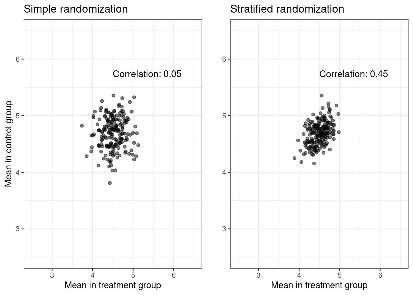
In the second plot, we simulate from the same DGP’s but change the variance of $X$, i.e., instead of $p_X = 0.5$, we use $p_X = 0.9$. The variance of $X$ is, of course, $p_X(1 - p_X)$ and is maximized when $p_X = 0.5$.

By using a smaller variance and therefore a more skewed distribution of sex, we observe a lower correlation. This follows since the variance in the amount of women in each treatment group is overshadowed by the fixed individual variance.

Conclusion

The above shows that stratified randomization induces a dependence structure in the data. More specifically, the iid. assumption of the observed data no longer holds, as the outcomes within the different strata are correlated. This poses a lot of problems, but luckily, more information leads to more certainty, so we can gain statistical efficiency by correctly taking the randomization procedure into account when modelling. I will explore the consequences for modeling in an upcomming blog post.

References

Kahan, Brennan C, and Tim P Morris. 2012. “Improper Analysis of Trials Randomised Using Stratified Blocks or Minimisation.” Statistics in Medicine 31 (4): 328–40.

--- title: "Stratified Randomization" date: "2024-01-07" bibliography: biblo.bib format: html: code-fold: true code-tools: true --- In my thesis I studied stratified randomization and it's consequences for modelling. In this post I will try to distill some of my work. This first blog post describes stratified randomization and its conseqeunces for modelling. # Randomization In a clinical trial, we want to single out the causal effect of treatment on the outcome. One way of ensuring that we can estimate a causal effect is by randomizing treatment to the study participants to balance the baseline covariates across treatment groups on average. That is, we aim for the two treatment groups to be comparable in all matters except treatment. There are many ways of randomizing treatment, but the simplest is to flip a fair coin to allocate treatment each time a participant enrolls in a study. This works well for large studies, but for small studies, there can be a significant risk of an imbalanced treatment allocation. To avoid this, we may enforce balance by using blocked randomization. Blocked randomization works by choosing an even number $k$ and then allocating treatment by drawing a random permutation of $k/2$ treated and $k/2$ controls for every $k$ participants enrolling in your study. The block size $k$ is typically chosen to be 4, 6, 8, or randomized among these. But even when treatment is forced to be balanced at all times, covariate imbalance across treatment is only guaranteed in expectation, and this may yield serious consequences for inference. In the extreme case, we may allocate all males to control and all females to treatment, but even in the non-extreme case, a large imbalance across treatment for a variable that is prognostic of the outcome can mar the purpose of randomization and lead to unnecessary uncertainty. Nearly all clinical trials conducted across various locations stratify by site to facilitate easier administration and data management. Additionally, many of these trials also stratify based on other baseline variables. ## Stratified Randomization Stratified randomization solves the issue of covariate imbalance by stratifying the randomization onto levels of certain prognostic baseline covariates. These levels are called strata. As an example, you might use blocked randomization within males and females separately to balance the distribution of sex across treatment, and typically, you only stratify on a few variables. To observe the consequences of stratified randomization for modeling, we posit the following trial in which we expect sex to be prognostic of the outcome and randomize patients within sex using blocked randomization. Let $Y$ denote the continuous outcome, $X$ denote sex, and $A$ denote a binary treatment variable where we target a 1:1 allocation. Inspired by [@kahan2012improper] we posit the following DGP's. For each $i = 1, \dots, 100$, let \begin{align*} &X_i \sim \text{Bernoulli}(1/2)\\ &A_i \sim \text{Bernoulli}(1/2)\\ &Y_i \mid X_i, A_i \sim \alpha + \beta_A A_i + \beta_X X_i \end{align*} and \begin{align*} &X_i \sim \text{Bernoulli}(1/2)\\ &A_i \sim \text{Stratified block randomization on } X \text{ with a block size of 4} \\ &Y_i \mid X_i, A_i \sim \alpha + \beta_A A_i + \beta_X X_i \end{align*} In the figure below, we simulate $N = 200$ datasets, each of size $n = 100$ with parameters $(\alpha = 0, \beta_A = 0.2, \beta_X = 0.5)$, and plot the treatment specific means against each other. ```{r} #| warning: false # Kahan, B. C., & Morris, T. P. (2011). Improper analysis of trials randomised # using stratified blocks or minimisation. Statistics in Medicine, 31(4), # 328–340. doi:10.1002/sim.4431 library(tidyverse) library(blockrand) library(patchwork) library(gridExtra) # Number of datasets N = 200 # Size of each dataset n_size = 100 sim_data = function(n_size, rand_type = 0, pX = 0.5) { # Simulate binary baseline covariate / the balancing variable sex = rbinom(n_size, 1, pX) # Simple randomization A_simple = rbinom(n_size, 1, 0.5) # Stratified Randomization A_strat = rep(0,n_size) n1 = sum(sex == 1) n0 = sum(sex == 0) A_strat[sex == 1] = as.numeric(blockrand(n=n1, num.levels=2)$treatment, block.sizes = 4)[1:n1]-1 A_strat[sex == 0] = as.numeric(blockrand(n=n0, num.levels=2)$treatment, block.sizes = 4)[1:n0]-1 # Simulate outcome outcome Y_simple = 0.2 * A_simple + 5 * sex + rnorm(n_size, sd = 1) Y_strat = 0.2 * A_strat + 5 * sex + rnorm(n_size, sd = 1) if (rand_type == 0) { c(mean(Y_simple[A_simple == 0]), c(mean(Y_simple[A_simple == 1]))) } else { c(mean(Y_strat[A_strat == 0]), c(mean(Y_strat[A_strat == 1]))) } } # Create a function to calculate correlation and annotate the plot annotate_corr = function(cor_val, x, y) { annotate("text", x = x, y = y, label = sprintf("Correlation: %.2f", cor_val), hjust = 0, vjust = 1, size = 4) } # Simulate 200 datasets of size 50 #set.seed(123) vec_simple = replicate(N, sim_data(n_size)) vec_strat = replicate(N, sim_data(n_size, rand_type = 1)) # Collect data into tibbles simple_df = tibble(Y0 = vec_simple[1, ], Y1 = vec_simple[2, ]) strat_df = tibble(Y0 = vec_strat[1, ], Y1 = vec_strat[2, ]) # Estimate the correlation cor_simple = cor(simple_df$Y0, simple_df$Y1) cor_strat = cor(strat_df$Y0, strat_df$Y1) p_simple = simple_df %>% ggplot() + geom_point(aes(x = Y0, y = Y1), alpha = 0.5) + theme_bw() + xlab("Mean in treatment group") + ylab("Mean in control group") + ggtitle("Simple randomization") + xlim(0, 5) + ylim(0, 5) + annotate_corr(cor_simple, 2.5, 4.8) p_strat = strat_df %>% ggplot() + geom_point(aes(x = Y0, y = Y1), alpha = 0.5) + theme_bw() + xlab("Mean in treatment group") + ylab("") + ggtitle("Stratified randomization") + xlim(0, 5) + ylim(0, 5) + annotate_corr(cor_strat, 2.5, 4.8) grid.arrange(p_simple, p_strat, ncol = 2) ``` Now we change the distribution of the binary baseline covariate $X$, i.e., \begin{align*} &X \sim \text{Bernoulli}(0.9)\\ \end{align*} to make the distribution of sex more skewed. This yields ```{r} #set.seed(123) vec_simple = replicate(N, sim_data(n_size, pX = 0.9)) vec_strat = replicate(N, sim_data(n_size, rand_type = 1, pX = 0.9)) # Collect data into tibbles simple_df = tibble(Y0 = vec_simple[1, ], Y1 = vec_simple[2, ]) strat_df = tibble(Y0 = vec_strat[1, ], Y1 = vec_strat[2, ]) # Estimate the correlation cor_simple = cor(simple_df$Y0, simple_df$Y1) cor_strat = cor(strat_df$Y0, strat_df$Y1) p_simple = simple_df %>% ggplot() + geom_point(aes(x = Y0, y = Y1), alpha = 0.5) + theme_bw() + xlab("Mean in treatment group") + ylab("Mean in control group") + ggtitle("Simple randomization") + ylim(2.5, 6.5) + xlim(2.5, 6.5) + annotate_corr(cor_simple, 4.5, 5.8) p_strat = strat_df %>% ggplot() + geom_point(aes(x = Y0, y = Y1), alpha = 0.5) + theme_bw() + xlab("Mean in treatment group") + ylab("") + ggtitle("Stratified randomization") + ylim(2.5, 6.5) + xlim(2.5, 6.5) + annotate_corr(cor_strat, 4.5, 5.8) grid.arrange(p_simple, p_strat, ncol = 2) ``` The non-zero correlation between the treatment-specific means in the case of stratified randomization arises from the fact that we force an equal distribution of $X$ within each treatment arm. If $X$ denotes sex (0: man, 1: woman), and if, by chance, we observe more women than men, stratified block randomization ensures more women than men within each treatment group. Since being a woman has a strong positive effect on the outcome, both treatment means will be larger. This is not the case for simple randomization. In the second plot, we simulate from the same DGP's but change the variance of $X$, i.e., instead of $p_X = 0.5$, we use $p_X = 0.9$. The variance of $X$ is, of course, $p_X(1 - p_X)$ and is maximized when $p_X = 0.5$. By using a smaller variance and therefore a more skewed distribution of sex, we observe a lower correlation. This follows since the variance in the amount of women in each treatment group is overshadowed by the fixed individual variance. # Conclusion The above shows that stratified randomization induces a dependence structure in the data. More specifically, the iid. assumption of the observed data no longer holds, as the outcomes within the different strata are correlated. This poses a lot of problems, but luckily, more information leads to more certainty, so we can gain statistical efficiency by correctly taking the randomization procedure into account when modelling. I will explore the consequences for modeling in an upcomming blog post.